There is a quiet revolution happening on Apple Silicon and it is not happening in San Francisco or Bangalore. It is happening right on your desk, inside a MacBook (any Chip like Pro with an M5 Pro chip and 24 GB of unified memory). A few years ago, running a model with 235 billion parameters, the kind of AI that powers the most advanced chatbots in the world, would have required a server room full of NVIDIA GPUs, liquid cooling and an electricity bill that could fund a small wedding in Kerala. Today, thanks to a technique called TurboQuant-MLX, that same model can sit inside your laptop and answer questions about Munnar tea estates or Alleppey backwaters while you sip your morning chai.
This article is written for the curious beginner, the developer who has heard the buzzwords but wants to understand what is actually happening under the hood. We will walk through what TurboQuant-MLX is, why it matters for your 24 GB MacBook Pro, how fast it really runs and we will write some simple Python code together to see it in action, using Kerala tourism as our playground.
1. Why MLX Exists
Before we talk about TurboQuant, we need to talk about MLX. Many developers have never heard of it and that is a shame because it is the engine that makes everything possible on your Mac.
MLX is Apple’s own machine learning framework, built from the ground up for Apple Silicon. It is not a wrapper around PyTorch and it is not a port of TensorFlow. It is a native framework that understands the M-series chips at a fundamental level.
If you have ever tried running large models with PyTorch on a Mac, you have probably felt the pain. PyTorch was built for NVIDIA CUDA GPUs. When you run it on a Mac, it falls back to the CPU or uses limited Metal support through third-party backends. The result is slow inference, high memory overhead and a lot of frustration. MLX, on the other hand, speaks the native language of the M5 Pro’s GPU. It compiles Metal kernels just-in-time, manages memory with zero-copy tensor sharing between CPU and GPU and treats unified memory as a single pool rather than two separate banks that need constant synchronization.
2. The Secret Weapon: Unified Memory
This is probably the most important concept to understand about Apple Silicon and it is the reason why a 24 GB Mac can do things that a traditional PC with 32 GB RAM and a dedicated GPU simply cannot.
On a traditional Windows or Linux machine, your CPU has its own RAM, say 32 GB and your GPU has its own VRAM, say 8 GB or 12 GB. When you run an AI model, the model weights must be copied from CPU RAM into GPU VRAM. If your model needs 20 GB, but your GPU only has 8 GB, you are stuck. You either need a bigger GPU or you run the model on the CPU, which is painfully slow. The CPU and GPU live in separate memory worlds and crossing that boundary costs time and bandwidth.
Apple Silicon changes this entirely. On your M5 Pro MacBook Pro, the CPU and GPU share the same physical memory pool. There is no CPU RAM and GPU VRAM. There is just memory, 24 GB of it and both the CPU and GPU can access it simultaneously without copying anything. MLX takes full advantage of this. When you load a model, MLX places the weights in unified memory and the GPU can read them directly. If the model is 20 GB, you still have 4 GB left for the operating system, the KV cache and MLX’s workspace. On a traditional PC with 32 GB RAM and an 8 GB GPU, that same 20 GB model would be impossible to run on the GPU and running it on the CPU would be a crawl.
This is why Apple Silicon punches so far above its weight class for local AI. The unified memory architecture removes the VRAM bottleneck that plagues every other platform.
3. The Problem: Why Big AI Models Refuse to Fit
Imagine you have a massive library. Not a small town library, but the British Library, with 235 billion books. Now imagine you want to carry that entire library inside your MacBook. That is roughly what we are trying to do when we run a large language model (LLM) like Qwen3-235B. These models are essentially enormous matrices of numbers, weights, that have been trained on vast amounts of text. In their original form, these weights are stored as 16-bit floating point numbers (BF16). A 235-billion-parameter model at BF16 precision needs roughly 470 GB of memory just to hold the weights. Your MacBook Pro has 24 GB. The math does not add up.
This is where quantization comes in. Quantization is the art of shrinking these numbers. Instead of storing each weight as a 16-bit number, we store it with fewer bits, maybe 3 bits or 4 bits. The challenge is doing this without making the model so dumb that it starts speaking gibberish. Traditional methods, like simple affine quantization, often break down at very low bit widths. The model becomes incoherent, hallucinates or simply forgets what it was asked.
4. What is TurboQuant-MLX?
TurboQuant-MLX is an implementation of Google’s TurboQuant research (Zandieh et al., 2025) built specifically for Apple’s MLX framework on Apple Silicon. Think of MLX as Apple’s native machine learning engine, designed to squeeze every ounce of performance out of the M-series chips. TurboQuant-MLX takes this a step further by applying extreme compression to both the model weights and something called the KV cache, which we will explain shortly.
At its heart, TurboQuant uses a beautifully simple two-step process:
Step 1: Hadamard Rotation. Before compressing the weights, TurboQuant multiplies them by a special mathematical matrix called a Hadamard matrix. This is like spinning a kaleidoscope before taking a photograph. The rotation spreads the information evenly across all dimensions, transforming any wild, irregular distribution of weights into something that looks almost like a smooth bell curve, a Gaussian distribution. This is data-oblivious, meaning it does not need any sample data to calibrate itself. It just works, mathematically, every time.
Step 2: Lloyd-Max Codebook Quantization. Once the weights are nicely distributed, TurboQuant applies Lloyd-Max quantization. This is an information-theoretically optimal method for quantizing Gaussian-distributed data. Instead of using simple linear buckets, it uses carefully computed codebooks that minimize the error for each bit width. The result is that even at 3 bits per weight, the model retains remarkable coherence and accuracy.
What makes TurboQuant-MLX special is that it does not stop at weight compression. It also compresses the KV cache at runtime, which is often the hidden memory killer in long conversations.
5. TurboQuant vs GGUF: Why This Is Not Just Another Ollama Format
If you have used Ollama before, you are probably familiar with GGUF, the quantization format that powers llama.cpp. It is natural to ask: is TurboQuant just another GGUF variant? The answer is no and the differences matter.
GGUF is a container format designed primarily for llama.cpp, which runs inference on both CPU and GPU across many platforms. It uses standard quantization techniques like Q4_0, Q5_K_M and Q8_0, which are essentially linear scaling methods that map floating point weights to low-bit integers. These work well for many models, but they struggle at very aggressive bit widths like 2-bit or 3-bit, especially on large Mixture-of-Experts models. At 3-bit, GGUF often produces noticeably degraded output and at 2-bit it typically collapses entirely.
TurboQuant is fundamentally different. It is not a container format. It is a quantization algorithm with three key innovations that GGUF does not have:
Hadamard Rotation. GGUF does not rotate weights before quantizing. TurboQuant does and this rotation is what allows the Lloyd-Max codebooks to work so effectively. Without rotation, the weight distribution is irregular and simple linear quantization wastes precision on unimportant values while starving important ones.
Lloyd-Max Codebooks. GGUF uses uniform or simple piecewise-linear quantization. TurboQuant uses mathematically optimal codebooks computed for Gaussian distributions. At 3-bit, this produces output quality that rivals 4-bit GGUF, while being significantly smaller.
KV Cache Compression and Expert Streaming. GGUF has no built-in mechanism for compressing the KV cache at runtime, nor does it support paging experts from disk for MoE models. TurboQuant-MLX does both, which is why a 235B model can run on a 24 GB MacBook Pro at all.
Here is a simple comparison to make the distinction clear:
Ollama remains excellent for quickly trying models and for developers who want a simple, cross-platform experience. TurboQuant-MLX is for the developer who wants to push Apple Silicon to its absolute limit, who needs to run models that simply will not fit under any other quantization scheme and who values the tight integration with MLX’s unified memory architecture.
6. Where TurboQuant Sits in Your AI Stack
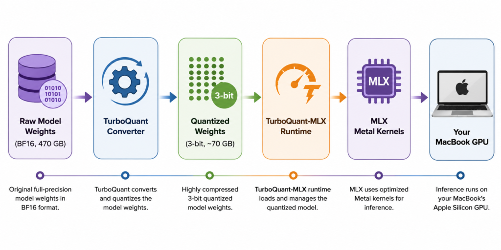
TurboQuant-MLX is not a replacement for your entire AI pipeline. It is a specialized compression and inference layer that sits between your model weights and the MLX runtime. Think of it as a highly optimized gearbox for Apple Silicon.
Here is where it fits:
The converter is a one-time step. You run it once to compress the model and then you use the quantized weights for every inference. The runtime handles dequantization on the fly during generation, compresses the KV cache as the conversation grows and streams experts from disk when memory is tight.
7. When NOT to Use TurboQuant
TurboQuant is powerful, but it is not the right tool for every job. Here are situations where you should probably look elsewhere:
You need maximum speed on small models. If you are running a 7B or 13B model that fits comfortably in memory at 4-bit, standard MLX quantization or even Ollama will be faster. TurboQuant’s Hadamard rotation and codebook lookup add a small overhead that is worth paying for extreme compression, but not for models that already fit easily.
You are not on Apple Silicon. TurboQuant-MLX is built exclusively for MLX and Metal. It will not run on NVIDIA GPUs, AMD GPUs or x86 CPUs. If your machine is not a Mac with an M-series chip, this is not for you.
You need exact numerical precision. At 3-bit and especially 2-bit, quantization introduces small errors. For most text generation, these errors are imperceptible. But if you are doing tasks where every digit matters, like precise financial calculations or cryptographic operations, you should use higher precision or verify outputs carefully. The full 3-bit sibling of the hybrid model passes stress tests for reasoning and coding, but exact literal recall can occasionally slip a digit.
You want a plug-and-play experience. Ollama wins here. Download, run, done. TurboQuant requires more setup: converting models, tuning cache budgets, possibly raising Metal memory limits. It rewards the developer who wants control and performance, not the one who wants zero configuration.
Your model is not supported. TurboQuant-MLX supports LLaMA, Qwen, Mistral, GPT-OSS, Nemotron and DeepSeek architectures. If you have a niche or legacy model outside these families, you will need to wait for support or use a different runtime.
8. Where TurboQuant Is Actually Useful
It is easy to get lost in the technical details and forget why any of this matters. Here are concrete scenarios where TurboQuant-MLX changes what is possible:
Local AI Assistants. Run a 122B or 235B model as your personal assistant. Your conversations stay on your machine. No API keys, no subscription fees, no data leaving your laptop. Ask it to summarize documents, draft emails or debug code, all offline.
Offline Coding Assistants. Connect a TurboQuant model to Cursor or VS Code via the OpenAI-compatible API. A 27B or 35B coder model running locally can suggest completions, refactor code and explain algorithms without sending your proprietary codebase to a third party.
RAG Applications. Retrieval-Augmented Generation systems need a capable language model to synthesize answers from retrieved documents. Running the generator locally with TurboQuant means your private documents never touch an external API.
Banking Applications. In the BFSI sector, regulatory compliance often forbids sending customer data to cloud AI services. A locally running 235B model can analyze transaction patterns, generate compliance reports and assist with risk assessment while keeping every byte of data inside your organization’s walls.
Healthcare AI. Medical records, diagnostic images and patient histories are among the most sensitive data there is. A local model can assist with clinical documentation, literature review and preliminary diagnosis support without exposing PHI to external servers.
Government AI. For defense, intelligence and public sector use cases where data sovereignty is law, local inference is not a preference, it is a requirement. TurboQuant makes frontier-grade models feasible on standard government-issue hardware.
Private Enterprise Chatbots. Companies can deploy internal knowledge bases and support bots without worrying about data leakage. The model lives on a Mac mini or MacBook Pro in the office, not in someone else’s data center.
Research. Academics and independent researchers can experiment with frontier models without needing grant funding for cloud compute. Reproduce papers, test hypotheses and build prototypes on hardware you already own.
9. The KV Cache: Why It Matters and How TurboQuant Handles It
To understand why KV cache compression is a big deal, you need to understand what the KV cache actually is. When a language model generates text, it does not read the entire conversation from scratch for every new word. That would be impossibly slow. Instead, it caches the intermediate computations from previous tokens in two matrices: the Key (K) matrix and the Value (V) matrix. Together, these are the KV cache.
Think of it like this. When you are reading a long novel, you do not go back to page one every time you start a new page. You remember what happened before. The KV cache is the model’s memory of what has already been said. The problem is that this memory grows linearly with the conversation length. A 131,000-token context on a 120B model can consume 45 MB per token position in FP16, which adds up to several gigabytes of memory. On a 24 GB machine, that cache can crowd out the model weights and crash the system.
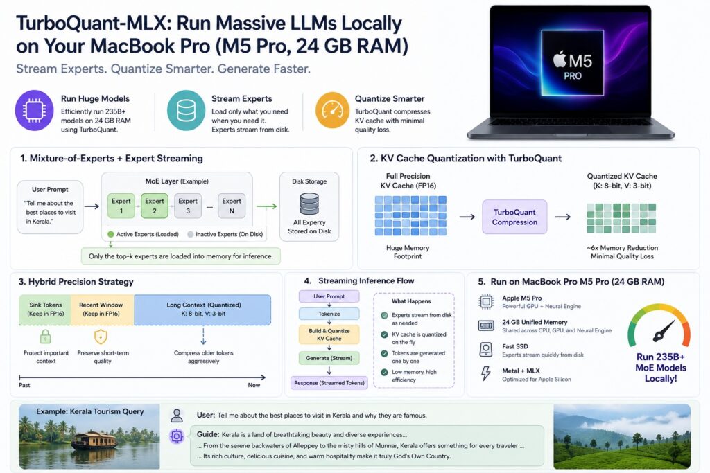
TurboQuant-MLX attacks this problem by compressing the KV cache at runtime using the same Hadamard rotation and Lloyd-Max codebook approach it uses for weights. But it goes further with mixed precision: it keeps the Key matrix at 8-bit precision, because keys are sensitive to error and compresses the Value matrix to 3-bit, because values tolerate more aggressive quantization. It also protects the first 128 tokens, called attention sinks, by keeping them in full FP16 precision. These early tokens anchor the model’s attention and must not be corrupted.
The result is a KV cache that is roughly four times smaller, with virtually no perceptible quality loss. On large models like GPT-OSS-120B, this compression is so effective that it actually speeds up generation, because the time saved by reading less memory outweighs the time spent decompressing. On smaller models, it is primarily a memory saver that lets you fit longer conversations into limited RAM.
Why MoE Models Benefit the Most
Mixture-of-Experts models are where TurboQuant truly shines and it comes down to simple arithmetic. A dense model like Qwen3.6-27B has 27 billion parameters and every single one is active for every token. There is no way around loading the whole thing. An MoE model like Qwen3-235B has 235 billion parameters, but only 22 billion are active per token. The other 213 billion are specialist experts that sit idle most of the time.
TurboQuant’s expert streaming exploits this sparsity. Instead of keeping all 128 experts in memory, it loads only the 8 that the router selects for the current token. The remaining 120 experts stay on disk. Because language has structure, the same experts tend to be reused across related tokens, so an LRU cache keeps the hot ones in memory. On a 24 GB Mac, this means you can run a model whose total weight footprint is 70 GB, because you only ever need a fraction of it in RAM at any moment.
Dense models cannot do this. Every parameter is active, so every parameter must be resident. MoE models, combined with TurboQuant’s streaming, break the RAM barrier in a way that dense models never can.
10. Your Setup: Qwen3-235B on Your MacBook
Let us talk specifically about your machine. If you have a MacBook Pro with an M5 Pro chip and 24 GB of unified memory. The Qwen3-235B-A22B model is a Mixture-of-Experts (MoE) architecture. This means it has 235 billion total parameters, but only about 22 billion are active for any given token. It is like a hospital with 128 specialist doctors, but for each patient, only 8 doctors are called into the room. This sparsity is what makes MoE models so powerful yet so tricky to run.
Here is the reality check for your 24 GB machine:
The full 3-bit quantized version of Qwen3-235B sits at about 103 GB on disk and needs roughly that much peak memory to run fully resident. That will not fit in 24 GB. The hybrid version, which uses 3-bit attention and 2-bit experts, shrinks to about 70.5 GB. Still too large for full residency.
However, TurboQuant-MLX offers a feature called expert streaming. This is where the magic happens for your machine. Instead of loading all 128 experts into memory at once, the system pages only the 8 experts that the router selects for each token, directly from your SSD. An LRU cache keeps recently used experts in memory, so if the model keeps calling the same specialists, they stay warm. On a 24 GB MacBook Pro, you would run this in streaming mode with a tight cache budget.
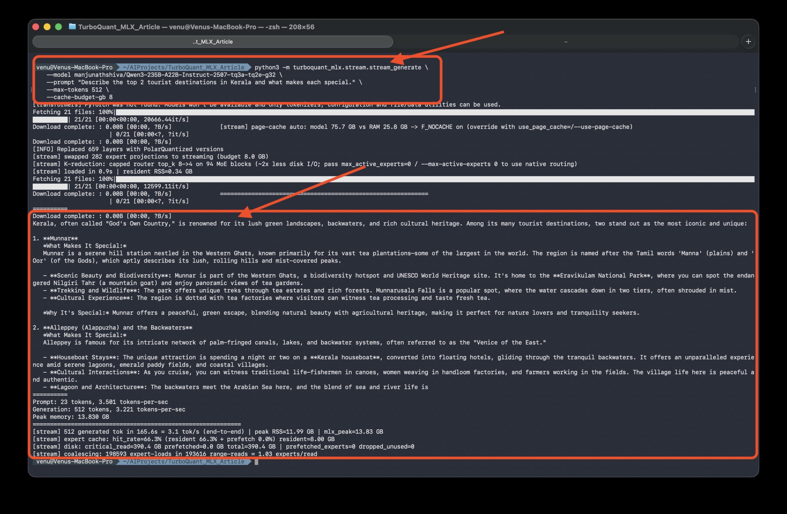
On a 16 GB Mac mini, the Qwen3-235B hybrid streams at roughly 0.2 tokens per second with a 6 GB cache budget. On your 24 GB M5 Pro, you can afford a larger cache budget, perhaps 8 to 10 GB, which should push your hit rate higher and your speed closer to 0.5 to 1 token per second. It is not blazing fast, but it is a 235-billion-parameter AI running on a laptop. That is the point.
11. Speed: What to Expect on Your M5 Pro
Let us ground the numbers in reality. The M5 Pro with 24 GB is a new tier that sits between the 16 GB Mac mini and the 48 GB or 64 GB MacBook Pros. Here is what the benchmarks tell us:
For smaller models that fit fully resident, the M5 Pro shines. The Qwen3.6-35B-A3B model, which is about 35 billion parameters with 3 billion active, runs at roughly 52 tokens per second when fully resident at 3-bit quantization. The Nemotron-3-Super-120B runs at about 20 tokens per second on a 48 GB machine when resident.
For your Qwen3-235B, the speed is dictated by disk bandwidth, not compute. The M5 Pro’s SSD is fast, but every token may need to fetch hundreds of megabytes of expert weights from disk. With expert streaming and parallel prefetching, the system tries to hide this latency. On your 24 GB machine, expect the model to be usable for thoughtful, deep reasoning tasks rather than rapid-fire chat. Think of it as having a very wise professor who takes a moment to compose each sentence, rather than a chatty friend.
The KV cache compression also plays a role. On large models like GPT-OSS-120B, compressing the KV cache to 3-bit actually makes generation faster (8.7 tok/s vs 6.4 tok/s) because the memory bandwidth saved outweighs the dequantization cost. On smaller active-parameter models, it is more of a memory saver than a speed booster.
12. Getting Started: Installation and First Steps
Let us get our hands dirty. First, install the package. Open your terminal and run: